Here’s how you can highlight duplicates in Excel using Conditional Formatting, along with an example table and instructions:
| ID | Name | Department | |
| 1 | Stefan | Marketing | Stefan.mail@gmail.com |
| 2 | Bob Johnson | Sales | bob.johnson@gmail.com |
| 3 | Stefan | Marketing | Stefan.mail@gmail.com |
| 4 | Carol White | IT | carol.white@example.com |
| 5 | Stefan | Marketing | Stefan.mail@gmail.com |
In this table:
- The Name column has duplicate entries for “Stefan”
- The Email column also has duplicate entries for “Stefan.mail@gmail.com”
Steps to Highlight Duplicates in Excel
- Select the Data Range:
- Highlight the range of cells you want to check for duplicates. In this case, select
B2:D6(Name, Department, and Email columns).
- Highlight the range of cells you want to check for duplicates. In this case, select
- Open Conditional Formatting:
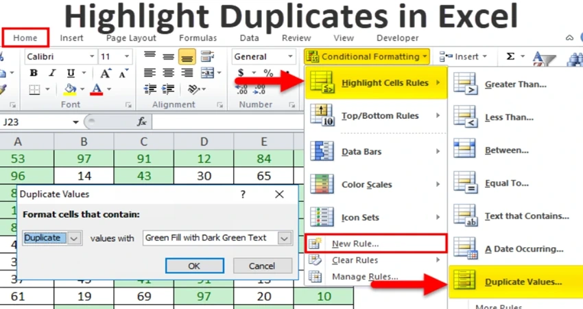
- Go to the Home tab on the ribbon.
- Click Conditional Formatting > Highlight Cells Rules > Duplicate Values.
- Choose Formatting Style:
- In the Duplicate Values dialog box, choose the formatting style (e.g., light red fill with dark red text).
- Click OK:
- Excel will highlight all duplicate values in the selected range.
Read Also: Best anthropology teacher for UPSC