Method to Determine Thermal Conductivity

The thermal conductivity of a material is determined by following methods

  1. Lee’s disc method – for bad conductors
  2. Radial flow method – for bad conductors

Lee’s Disc Method

Definition:

Lee’s disc method is an accurate method of measuring the thermal conductivity of poor conductor capable of giving results over a wide range of temperatures.

Description:
  • The Lee’s disc apparatus consists of two thin discs A and C.
  • The entire arrangements can be suspended from an iron stand.
  • The specimen (bad conductor i.e., glass or card board) under test is taken in the form of a thin sheet B and placed between a copper disc C and a hollow cylinder A.
  • The specimen has the same diameter as A or C. Holes are drilled near the bottom of A and the middle of C to take thermometer T1 and T2.
  • These will indicate the temperatures of the faces of the specimen when the steady state is reached.
  • The metal apparatus are chromium or nickel plated so that they will have the same emissive powers.
Lee's disc apparatus
Fig. (A) Lee’s disc apparatus
Working:
Steam is passed through the cylinder A continuously for the same time until the thermometers T1 and T2 show steady temperatures. Let θ1 and θ2 be the temperature shown by T1 and T2 in the steady state. The quantity of heat Q conducted a cross the specimen per sec is equal to the quantity emitted from the exposed surface of the metal slab C per second.
Thus,
eqn (1)
\mathrm{Q}=\mathrm{k} \pi \mathrm{r}^{2}\left(\frac{\theta_{1}-\theta_{2}}{\mathrm{~d}}\right)
Where, r is the radius of the slab C and d its thickness.

Now, the specimen is removed and the cylinders A and C are kept in contact, while steam is still passing through A until the temperature of the slab C rises by  8°C above the steady state temperature θ2. Now the upper cylinder A, is removed and C is exposed to the surrounding and allowed to cool. The temperature of the slab for every half a minute in recorded and a cooling curve is drawn as shown in (Fig. B). From this curve, the rate of cooling   \left(\frac{\mathrm{d} \theta}{\mathrm{dt}}\right)  given by the slope of the cooling curve at the steady temperature of the slab C (i.e) θ2 is determined.

Cooling Curve
Fig. (B) Cooling curve

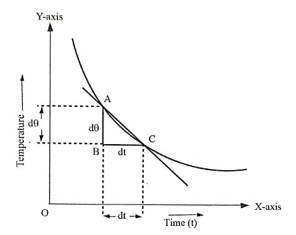
Now, the heat lost by radiation from the top and bottom and curved surface of the disc C is proportional to the area, 2πr2 + 2πrd.

Where r is the radius of the slab C and d is its thickness.

Since \frac{d \theta}{d t}   gives the rate of cooling, the rate of loss of heat is MS \frac{d \theta}{d t}

Where M is the mass of the disc C,

S is the specific heat.

In the first part of the experiment the total exposed surface area is (πr2+2πrd) and the heat radiated by this exposed area is given by

\mathrm{Q}=\frac{\pi \mathrm{r}^{2}+2 \pi \mathrm{rd}}{2 \pi \mathrm{r}^{2}+2 \pi \mathrm{rd}} \mathrm{MS} \frac{\mathrm{d} \theta}{\mathrm{dt}}

This quantity of heat must be equal to the quantity of heat conducted through the specimen during the steady state given by

\mathrm{Q}=\mathrm{K} \pi \mathrm{r}^{2}\left(\frac{\theta_{1}-\theta_{2}}{\mathrm{~d}}\right)

Since they are equal,
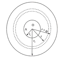
\begin{aligned} K \pi r^{2}\left(\frac{\theta_{1}-\theta_{2}}{d}\right) & =\frac{r+2 d}{2(r+d)} M S \frac{d \theta}{d t} \\ K & =\frac{M S \frac{d \theta}{d t} d(r+2 d)}{\pi r^{2}\left(\theta_{1}-\theta_{2}\right) 2(r+d)} \end{aligned}
Knowing the values of other quantities, K can be calculated.

Radial flow of heat

Definition:
The heat which is conducted radially through the pipe is known as radial flow of heat. Example, heat flow through refrigerator pipe, steam pipe etc.
 Spherical shell method
It is suitable for poor conductors like cork, charcoal, clay etc. The specimen in the powder from which is under test is contained between two thin spherical shells A and B of radius r1 and r2 respectively. A heating element is placed at the centre O of the shells. There is a radical flow heat from inner to the outer shell and subsequently lost by emission from the surface of the outer shell as shown in (Fig. C). Let K be the thermal conductivity of the specimen and θ1 and θ2 be the temperatures of the inner and outer shells respectively, when a steady state has been reached.
\mathrm{Q}=-\mathrm{K} 4 \pi \mathrm{r}^{2} \frac{\mathrm{d} \theta}{\mathrm{dr}}
Spherical Shell Method
Fig. (C) Spherical shell method
Consider a spherical shell of radius r and thickness dr having temperature θ and θ+dθ on its inner and outer surface respectively. The quantity of heat conducted per second through this shell is given by
\begin{aligned} \mathrm{Q}=-\mathrm{KA} \frac{\mathrm{d} \theta}{\mathrm{dr}} & =-\mathrm{K} 4 \pi \mathrm{r}^{2} \frac{\mathrm{d} \theta}{\mathrm{dr}}\left(\text { since } \mathrm{A}=\pi \mathrm{r}^{2}\right) \\ \frac{\mathrm{dr}}{\mathrm{r}^{2}} & =\frac{-4 \pi \mathrm{K}} \mathrm{Q}} \mathrm{d} \theta \end{aligned}
(i.e.)
Integrating between the limits r1 and r2 we get
\int_{\mathrm{r}_{1}}^{\mathrm{r}_{2}} \frac{\mathrm{dr}}{\mathrm{r}^{2}}=\frac{-4 \pi \mathrm{K}}{\mathrm{Q}} \int_{\theta_{1}}^{\theta_{2}} \mathrm{~d} \theta
\frac{1}{\mathrm{r}_{1}}-\frac{1}{\mathrm{r}_{2}}=\frac{4 \pi \mathrm{K}}{\mathrm{Q}}\left(\theta_{1}-\theta_{2}\right)
\mathrm{K}=\frac{\mathrm{Q}\left(\mathrm{r}_{2}-\mathrm{r}_{1}\right)}{4 \pi \mathrm{r}_{1} \mathrm{r}_{2}\left(\theta_{1}-\theta_{2}\right)}
Therefore,

Thus, the thermal conductivity K of the poor conductors can be calculated.

Read More Topics
Classification of dielectric materials
Applications of superconducting materials
Classification of nonlinear materials

About the author

Nandhini Sathish

View all posts

Leave a Reply