How to Pull Data from Another Sheet in Excel

Pull Data from Another Sheet: Excel is a powerful tool for organizing, analyzing, and presenting data. One of the most useful features in Excel is the ability to pull data from one sheet to another. Whether you’re working on a financial report, managing inventory, or creating dashboards, this functionality can save you time and reduce manual errors.

This tutorial will cover various methods for extracting data from another Excel sheet, along with an example.

Why Pull Data from Another Sheet?

Pulling data from another sheet in Excel allows you to:

Consolidate data from multiple sheets into one place.
Create dynamic reports that update automatically.
Organize data efficiently across multiple sheets.

Methods to Pull Data from Another Sheet

Here are three common methods for pulling data:

1. Using a Simple Reference Formula

The easiest way to pull data from another sheet is to use a reference formula.

Steps:

Go to the cell where you want the data to appear.
Type =.
Click on the sheet containing the source data.
Click on the specific cell you want to pull from.
Press Enter.

Example:

If you want to pull data from cell A1 in a sheet named “Sheet2” into cell A1 of

“Sheet1”:

=Sheet2!A1

2. Using the VLOOKUP Function

VLOOKUP is useful when you need to look up and pull data based on a matching value.

Steps:

Identify the unique identifier in both sheets.
Use the VLOOKUP formula:

=VLOOKUP(lookup_value, table_array, col_index_num, [range_lookup])

Example:

Imagine you have a product ID in “Sheet1” and want to pull the product name from “Sheet2”. If the product name is in column 2 of the table in “Sheet2”:

=VLOOKUP(A2, Sheet2!A1:B10, 2, FALSE)

3. Using the INDEX-MATCH Combination

INDEX-MATCH is a more flexible alternative to VLOOKUP.

Steps:

1. Use the MATCH function to find the row number:

=MATCH(lookup_value, lookup_array, 0)

2. Use the INDEX function to pull the data:

=INDEX(array, row_num, [column_num])

Example:

If you’re pulling a product name from “Sheet2” for a product ID in “Sheet1”:

=INDEX(Sheet2!B1:B10, MATCH(A2, Sheet2!A1:A10, 0))

Example Workbook

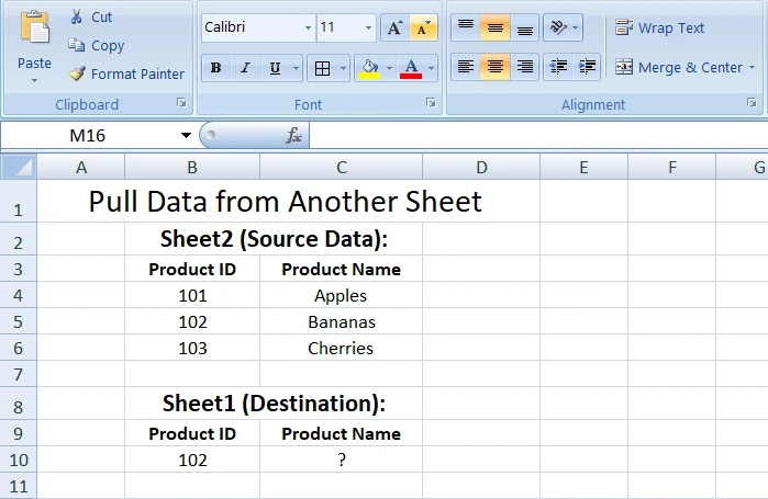
Imagine you have the following data:

Sheet2 (Source Data):

Product ID	Product Name
101	Apples
102	Bananas
103	Cherries

Sheet1 (Destination):

Product ID	Product Name
102	?

To pull the product name for Product ID 102 into “Sheet1”, you could use:

Reference Formula: =Sheet2!B2
VLOOKUP: =VLOOKUP(A2, Sheet2!A1:B10, 2, FALSE)
INDEX-MATCH: =INDEX(Sheet2!B1:B10, MATCH(A2, Sheet2!A1:A10, 0))

Tips and Best Practices

Use Named Ranges: Assign names to ranges for better readability, e.g., “ProductList” instead of “Sheet2!A1:B10”.
Check for Errors: Wrap formulas with IFERROR to handle missing data gracefully, e.g.,

=IFERROR(VLOOKUP(A2, Sheet2!A1:B10, 2, FALSE), "Not Found")

Keep Data Organized: Maintain a clear structure in your source sheets to simplify pulling data.

Learning how to pull data from another sheet in Excel is a valuable skill for improving efficiency and accuracy in your work. Whether you’re using a simple reference formula, VLOOKUP, or INDEX-MATCH, these methods will help you streamline your tasks. Try applying these techniques to your projects and experience the difference!