Control System Engineering and Mathematical Models

Intro Control System Engineering

Control system engineering theory evolved as an engineering discipline and due to universality of the principles involved, it is extended to various fields like economy, sociology, biology, medicine, etc. Control theory has played a vital role in the advance of engineering and science. The automatic control has become an integral part of modem manufacturing and industrial processes.

For example, numerical control of machine tools in manufacturing industries, controlling pressure, temperature, humidity, viscosity and flow in process industry. When a number of elements or components are connected in a sequence to perform a specific function, the group thus formed is called a system. In a system when the output’ quantity is controlled by varying the input quantity, the system is called control system. The output quantity is called controlled variable or response and input quantity is called command signal or excitation.

OPEN LOOP SYSTEM

Any physical system which does not automatically correct the variation in its output, is called an open loop system, or control system in which the output quantity has no effect upon the input quantity are called open-loop control system. This means that the output is not fedback to the input for correction. In open loop system the output can be varied by varying the input. But due to external disturbances the system output may change. When the output changes due to disturbances, it is not followed by changes in input to correct the output. In open loop systems the changes in output are corrected by changing the input manually.

CLOSED LOOP SYSTEM

Control systems in which the output has an effect upon the input quantity in order to maintain the desired output value are called closed loop systems. The open loop system can be modified as closed loop system by providing a feedback. The provision of feedback automatically corrects the changes in output due to disturbances. Hence the closed loop system is also called automatic control system. The general block diagram of an automatic control system is shown in image. It consists of an error detector, a controller, plant (open loop system) and feedback path elements.

The reference signal ( or input signal ) corresponds to desired output. The feedback path elements samples the output and converts it to a signal of same type as that of reference signal. The feedback signal is proportional to output signal and it is fed to the error detector. The error signal generated by the error detector is the difference between reference signal and feedback signal. The controller modifies and amplifies the error signal to-produce better control action. The modified error signal is fed to the plant to correct its output.

Advantages of open loop Control System Engineering

The open loop systems are simple and economical .
The open loop systems are easier to construct.
Generally the open loop systems are stable.

Disadvantage of open loop system

The open loop systems arc inaccurate and unreliable.
The changes in the output due to external disturbances are not corrected automatically.

Advantages of closed loop systems

The closed loop systems are accurate.
The closed loop systems are accurate even in the presence of non-linearities.
Sensitivity of the systems may be made small to make the system more stable.
The closed loop systems are less affected by noise.

Disadvantages of closed loop systems

The closed loop systems are complex and costly.
The feedback in closed loop system may lead to oscillatory response.
Feedback reduces the overall gain of the system.
Stability is a major problem in closed loop system and more care is needed to design a stable closed loop system.

EXAMPLES OF CONTROL SYSTEMS TEMPERATURE CONTROL SYSTEM

OPEN LOOP SYSTEM Engineering

The electric furnace shown in image. is an open loop system. The output in the system is the desired temperature. The temperature of the system is raised by heat generated by the heating element The output temperature depends on the time during which the supply to heater remains ON.

The ON and OFF of the supply is governed by the time setting of the relay. The temperature is measured by a sensor, which gives an analog voltage corresponding to the temperature of the furnace. The analog signal is converted to digital signal by an Analog – to – Digital converter (AD converter). The digital signal is given to the digital display device to display the temperature. In this system if there is any change in output temperature then the time setting of the relay is not altered automatically.

CLOSED LOOP SYSTEM

The electric furnace shown in image is a closed loop system. The output of the system is the desired temperature and it depends on the time during which the supply to heater remains ON.

The switching ON and OFF of the relay is controlled by a controller which is a digital system or computer. The desired temperature is input to the system through keyboard or as a signal corresponding to desired temperature via ports. The actual temperature is sensed by sensor and converted to digital signal by the A/D converter. The computer reads the actual temperature and compares with desired temperature. If it finds any difference then it sends signal to switch ON or OFF the relay through D/A converter and amplifier. Thus the system automatically corrects any changes in output. Hence it is a closed loop system.

EXAMPLE 2 : TRAFFIC CONTROL SYSTEM OPEN LOOP SYSTEM

Traffic control by means of traffic signals operated on a time basis constitutes an open-loop control system. The sequence of control signals are based on a time slot given for each signal. The time slots are decided based on a traffic study. The system will not measure the density of the traffic before giving the signals. Since the time slot does not changes according to traffic density, the system is open loop system.

CLOSED LOOP SYSTEM

Traffic control system can be made as a closed loop system if the time slots of the signals are decided based on the density of traffic. In closed loop traffic control system, the density of the traffic is measured on all the sides and the information is fed to a computer. The timings of the control signals are decided by the computer based on the density of traffic . Since the closed loop system dynamically changes the timings, the flow of vehicles will be better than open loop system.

EXAMPLE 3 : NUMERICAL CONTROL SYSTEM

OPEN LOOP SYSTEM

- Numerical control is a method of controlling the motion of machine components using of numbers. Here, the position of work head tool is controlled by the binary information contained in a disk.
- A magnetic disk is prepared in binary form representing the desired part P (P is the metal part to be machined).
- The tool will operate on the desired part P. To start the system, the disk is fed through the reader to the D/A converter. The D/A converter converts the FM(frequency modulated) output of the reader to a analog signal.
- It is amplified and fed to servomotor which positions the cutter on the desired part P.
- The position of the cutter head is controlled by the angular motion of the servornotor. This is an open loop system since no feedback path exists between the output and input.
- The system positions the tool for a given input command. Any deviation in the desired position is not checked and corrected automatically.

CLOSED LOOP SYSTEM

A magnetic disk is prepared in binary form representing the desired part P (P is the metal part to machined). To start the system, the disk is loaded in the reader. The controller compares the frequent modulated input pulse signal with the feedback pulse signal. The controller is a computer or microprocessor system. The controller carries out mathematical operations on the difference in the pulse signals and generates an error signal. The D/A converter converts the controller output pulse (error signal) into an analog signal.

The amplified analog signal rolates the servomotor to position the tool on the job. The position of the cutterhead is controlled according to the input of the servomotor. The transducer attached to the cutterhead converts the motion into an electrical signal. The analog electrical signal is converted to the digital pulse signal by the A/D converter.

Then this signal is compared with the input pulse signal. If there is any difference between these two, the controller sends a signal to the servomotor to reduce it. Thus the system automatically corrects any deviation in the desired output tool position. An advantage of numerical control is that complex parts can be produced with uniform tolerances at the maximum milling speed.

EXAMPLE 4 : POSITION CONTROL SYSTEM USING SERVOMOTOR

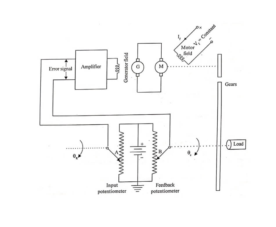
The position control system shown in servomotor powered by a generator. The load whose position has to be controlled is connected to motor shaft through gear wheels. Potentiometcrs are used to convert the mechanical motion to electrical signals.

The desired load position (0,) is set on the input potentiometer and the actual load position (0.) is fed to feedback potentiometer. The difference between the two angular positions generates an error signal, which is amplified and fed to generator field circuit. The induced emf of the generator drives the motor.

The rotation of the motor stops when the error signal is zero, i.e. when the desired load position is reached. 1.7 is a closed loop system. The system consists of a This type of control systems are called servomechanisms .The servo or servomechanisms are feedback control systems in which the output is mechanical position (or time derivatives of position e.g. velocity and acceleration).

MATHEMATICAL MODELS OF CONTROL SYSTEMS

A control system is a collection of physical objects (components) connected together to serve an

objective. The input output relations of various physical components of a system are governed by differential equations. The mathematical model of a control system constitutes a set of differential equations. The response or output of the system can be studied by solving the differential equations for various input conditions.

The mathematical model of a system is linear if it obeys the principle. of superposition and homogenity. This principle implies that if a system model has responses y,(t) and y, (t) to any inputs x, (t) and x, (t) respectively, then the system response to the linear combination of these inputs a, x, (t) + a, x, (t) is given by linear combination of the individual outputs a, y,(t)+a, y,(t), where a, and a, are constants. The principle of superposition can be explained diagrammatically as shown in image

A mathematical model will be linear if the differential equations describing the system has constant coefficients (or the coefficients may be functions of independent variables). If the coefficients of the differential equation deseribing the system are constants then the model is finear time invariant, If the coefficients of differential equations governing the system are functions of time then the model is lineu time varying.

The differential equations of a linear time invariant system can be reshaped into different form for the convenience of analysis. One such model for single input and single output system analysis is transfer function of the system. The transfer function of a system is defined as the ratio of Laplace transform of output to the Laplace transform of input with zero initial conditions.

Transfer function = Laplace Transform of output / Laplace Transform of input | with zero initial conditions..

The transfer function can be obtained by taking Laplace transform of the differential equations governing the system with zero initial conditions and rearranging the resulting algebraic equations to get the ratio of output to input.

MECHANICAL TRANSLATIONAL SYSTEMS

The model of mechanical translational Control system engineering can be obtained by using three basic elements mass, spring and dash-pot. These three elements represents three essential phenomena which occur in various ways in mechanical systems.

The weight of the mechanical system is represented by the clement mass and it is assumed to be concentrated at the center of the body. The elastic deformation of the body can be represented by a spring. The friction existing in rotating mechanical system can be represented by the dash-pot. The dash- pot is a piston moving inside a cylinder filled with viscous fluid. When a force is applied to a translational mechanical system, it is opposed by opposing forces due to mass, friction and elasticity of the system.

The force acting on a mechanical body are governed by Newton’s second law of motion. For translational systems it states that the sum of forces acting on a body is zero. (or Newton’s second law states, that the sum of applied forces is equal to the sum of opposing forces on a body).

LIST OF SYMBOLS USED IN MECHANICAL TRANSLATIONAL SYSTEM

x = Displacement, m.

v= dx/dt = Velocity, m/sec.

a = dv/dt = d²x/dt² = Acceleration, m/sec².

f = Applied force, N (Newtons).

f_m = Opposing force offered by mass of the body, N.

f_k= Opposing force offered by the elasticity of the body (spring), N.

f_b = Opposing force offered by the friction of the body (dash – pot), N.

M = Mass, kg.

K = Stiffness of spring, N/m.

B = Viscous friction co-efficient, N-sec/m.

Note : Lower case letters are functions of time.

Guideline to determine the Transfer Function of Mechanical Translational System

In mechanical translational system, the differential equations governing the system are obtained by writing force balance equations at nodes in the system. The nodes are meeting point of elements. Generally the nodes are mass elements in the Control system engineering. In some cases the nodes may be without mass element.
The linear displacement of the masses (nodes) are assumed as x₁, x₂, x₃, etc., and assign a displacement to each mass(node). The first derivative of the displacement is velocity and the second derivative of the displacement is acceleration.
Draw the free body diagrams of the Control system engineering. The free body diagram is obtained by drawing each mass separately and then marking all the forces acting on that mass (node). Always the opposing force acts in a direction opposite to applied force. The mass has to move in the direction of the applied force. Hence the displacement, velocity and acceleration of the mass will be in the direction of the applied force. If there is no applied force then the displacement, velocity and acceleration of the mass will be in a direction opposite to that of opposing force.
For each free body diagram, write one differential equation by equating the sum of applied forces to the sum of opposing forces.
Take Laplace transform of differential equations to convert them to algebraic equations. Then rearrange the s-domain equations to eliminate the unwanted variables and obtain the ratio between output variable and input variable. This ratio is the transfer function of the system.

Note: Laplace transform of x(t) = L{x(t)} = X(s) .

Laplace transform of dx(t)/dt = L{d/dt x(t)}= s X(s) (with zero initial conditions)

Laplace transform of d²x(t)/dt²⁼= L{d²/dt² x(t)}= s² X(s) (with zero initial conditions)