When the digital data transmitted from an information source to a destination, the output of a channel differs from its input because, the channel is subjected to various types of noise distortion and interference.
These additive noises will leads to an error. In order to avoid this, an error control is necessary. Such, error control mechanism involves both error detection and error correction.
NEED FOR CODING
- The main task required in digital communication system is to construct “Cost Effective System” for transmitting information from a sender (one end of the system) at a rate that is acceptable to a user (the other end of the system).
- The only practical option available to improve data quality is “Error Control coding”. The model of a digital communication system with channel coding is shown as,
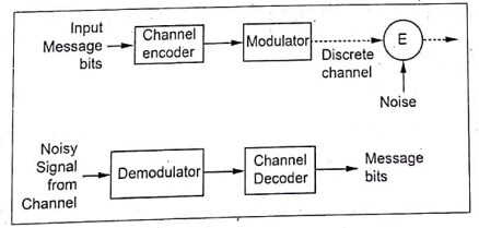
Fig 1.Digital Communication System with Channel Encoding
- The channel encoder adds extra bits to the message bits. The encoded signal is then transmitted over the noisy channel. The channel decoder identifies the redundant bits and uses them to detect and correct errors in the message bits if any.
- Thus the number of errors introduced due to channel noise is minimized by encoder and decoder. Due to the redundant bits, the overall data rate increases. Hence, channel has to accommodate this increased data rate. The system becomes slightly complex because of coding techniques.
- The error control code application areas are included: deep space communication, satellite communication, data transmission, data storage, mobile communication, file transfer, and digital audio/video transmission.
TYPES OF CODES
The codes are mainly classified as,
(a) Block Codes: It consists of ‘n’ number of bits in one block or codeword. This codeword consists of ‘ k ’ message bits and (n-k) redundant bits. Such block codes are called (n,k) block codes.
(b) Convolutional Codes: The coding operation is discrete time convolution of input sequence with the impulse response of the encoder. The Convolutional encoder accepts the message bits continuously and generates the encoded sequence continuously.
The codes are also been classified as,
(i) Linear Codes: If the two code words of the linear code are added by modulo -2 arithmetic, then it produces third codeword in the code.
(ii) Nonlinear Code : Addition of the nonlinear codewords does not necessarily produce third codeword.
METHODS OF CONTROLLING ERRORS
There are two main methods used for error control coding. They are,
(i) Forward Error Correction(FEC) – The errors are detected and corrected by proper coding techniques at the receiver. The check bits or redundant bits are used by the receiver to detect and correct errors.
Advantages: This method is faster.
Demerit : The overall probability of errors is higher. Since, some of the errors cannot be corrected.
(ii) Error Detection with Retransmission – The decoder checks the input sequence, when it detects any error, it discards that part of the sequence and requests the transmitter for retransmission. The transmitter then again transmits the part of the sequence in which error was detected.
Advantages: The overall probability of errors is low.
Demerit : This method is slower.
TYPES OF ERRORS
There are mainly two types of errors introduced during transmission of the data:
- Random Errors: These are the errors generated due to white guassian noise in the particular interval does not affect the performance of the system in the subsequent intervals. Normally these errors are uncorrelated. Therefore, it is called as random errors
- Burst Errors: These errors are generated due to impulsive noise in the channel. These impulse noise(bursts) are generated due to lightning and switching transients. These noise bursts affect several successive symbols. These errors are dependent on each other in successive message intervals. Hence, they are called as burst errors.
TERMS TO BE REMEMBERED IN ERROR CONTROL CODING
Code word: The encoded block of ‘n ’ bits is called a code word. It contains message bits and redundant bits.
Block length: The number of bits ‘n after coding is called the block length of the code.
Code rate: The ratio of message bits(k) and the encoder output bits(n) is called code rate. It is given as, ![\mathrm{r}=\left[\frac{k}{n}\right], 0<\mathrm{r}<1](https://pedagogyzone.com/wp-content/ql-cache/quicklatex.com-2988491b337731b4307a82507092fcce_l3.png "Rendered by QuickLaTeX.com") ….. eqn (1)
….. eqn (1)
![\mathrm{R}_0=\left[\frac{n}{k}\right], \mathrm{R}_{\mathrm{s}}](https://pedagogyzone.com/wp-content/ql-cache/quicklatex.com-1db4fe57dd468e970aef583cee72f72c_l3.png "Rendered by QuickLaTeX.com") …… eqn (2)
…… eqn (2)Code vectors: An ‘n ’ bit codeword can be visualized in an n-dimensional space as a vector whose elements or co-ordinates are the bits in the codeword. The following table gives various points as code vectors in the 3 -dimensional spaces.

Hamming Distance: The number of elements in which the two code vectors differ is said to be the Hamming distance.
Example: A = (111) and B = (010) .The two code vectors differ in first and third bits. Therefore, the hamming distance between A and B is ‘two’. It is denoted as d(A,B) or simply ‘d ’ .i.e.,
d(A,B) = d = 2
Thus, for 3 bit code vectors, the maximum hamming distance is 3 between (000) and (111).
Code Efficiency: The code efficiency is, “the ratio of message bits and ‘ n ’ transmitted bits.” and is given as,
Code efficiency ![\eta=\left[\frac{\text { Message bits in ablock }}{\text { Transmitted bits for the block }}\right]](https://pedagogyzone.com/wp-content/ql-cache/quicklatex.com-3b8bec5bb5534975cbc6ff6383519fac_l3.png "Rendered by QuickLaTeX.com")
Code efficiency ![\eta=\left[\frac{k}{\dot{n}}\right]=](https://pedagogyzone.com/wp-content/ql-cache/quicklatex.com-00f908cdb5aec0e546edc35f9d16e5cc_l3.png "Rendered by QuickLaTeX.com") Code rate …… eqn (4)
Code rate …… eqn (4)
Weight of the code: The number of non-zero elements in the transmitted code vector is called vector weight. It is denoted by w(A) , where is the code vector.
Example: if A = 1100 0001, the weight of this code vector will be w(A) = 3.
| Read More Topics |
| What is power system analysis? |
| Components and structure of electric power system |
| Advantages of per unit representation |